Weighted average is a calculation, which includes various degree of importance of values. From this article, you will learn how to calculate a weighted average in Excel by using the SUMPRODUCT and SUM formulas.
SUMPRODUCT formula
In one of my the previous articles, I have presented basic methods of calculating the arithmetic average, however, Excel unfortunately does not provide any special function for calculating weighted average. In such situation, we can use other available functions and one of the best for this purpose is SUMPRODUCT.
The SUMPRODUCT function is used to multiply values entered to data ranges and then sums them up. Syntax of this function is:
=SUMPRODUCT(array1; [array2]; [array3];…)
Array 1,2,3…. – these are arguments of the function and they define ranges of data that should be multiplied by each other and then results of multiplications are added.
How works SUMPRODUCT function?

In the example above, the arguments for the function are data ranges B2 to B7 and C2 to C7. The SUMPRODUCT function multiplies values from B2-B7 by the values from C2-C7, and then sums up the results (B2 * C2 + B3 * C3 + B4 * C4, etc.).
Important note:
Array arguments used in the SUMPRODUCT function must have the same size. In the situation, that one of the used tables is bigger or smaller than the other ones, the function will return the #VALUE! error, which indicates that formula has been typed incorrectly:

Examples for calculating weighted average
Below, I will show you two practical examples, in which you can use the function SUMPRODUCT and SUM to calculate the weighted average in Excel.
Example 1 – weights are summing up to 100%
A student during the semester received some grades for individual tasks, which have specific percentage weight assigned (the sum of weights is 100%):

Based on this information, we want to calculate the final grade, but due to different weights for individual grades, we can’t use the arithmetic average. By using the SUMPRODUCT function, we can calculate the sum of individual grades multiplied by their weights, so we get a weighted average:

Each value from column B was multiplied by the corresponding weight in column C, and then the results were added. Obtained result (3,75) is a weighted average, so the student’s grade should be 4 (rounded to the whole number).
The following picture shows that an identical result could also be received if we manually multiply each grade by the corresponding weight (results in column D, the formulas used in column E have been used) and add them:

Example 2 – weights are not summing up to 100% or are not percentage values
The example described above was quite simple, as the weights were percentage values and they summed up to 100%. However, what should we do, if the weights do not sum up to 100% or are not percentage? To calculate the weighted average in such situations, we should use a combination of two functions: SUM.PRODUCT and SUM.
In this example, we also want to calculate the final grade for the student, but the weights are expressed as numbers and their total is 15:

In this situation, we should first use SUMPRODUCT to multiply each grade by weight and add the results. The next step is diving received value by the sum of weights calculated by the SUM function:
=SUMPRODUCT(numbers(grades range); weights range)/SUM(weights range)
So, for our example correct formula should be entered as below:
=SUMPRODUCT(B2:B7; C2:C7)/SUM(B2:B7)

We have received information, that final grade for this student should be 4 (3,57 rounded to whole number).
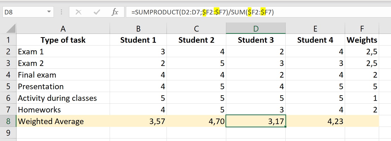
You can calculate weighted average for more than one student, but you have to make sure, that cells reference in formulas will be written correctly with $ sign: