By default, all data entered into cells in Excel are in general format, so it means that no particular number format is specified. However, very often we have to work with numbers that should be formatted in a specific way: as currency, percentage, fraction or a date.
To customize the data format, open the Format Cells dialog window – you can read more about cells formatting here. Data formatting commands are also quickly available on the Ribbon in the Home tab, in the Numbers group:

After clicking the arrow in the lower right corner of the Numbers group, a new window with data formatting options opens, in which you can find many available formats divided into categories:

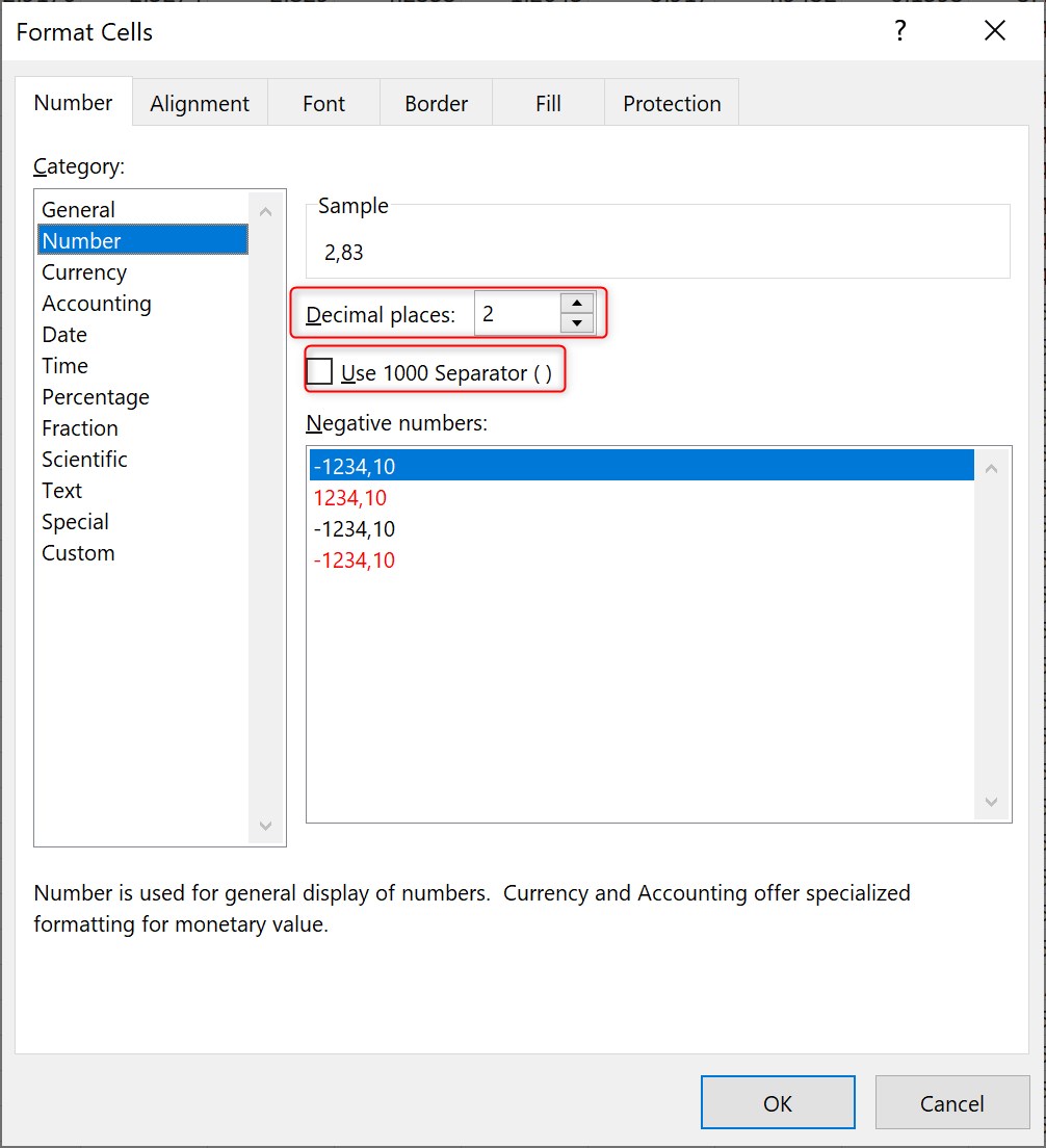
Number format – as the name suggests, it is used to format numeric values. Within this category, you can add a 1000 separator, specify how many decimal numbers should be displayed in the cell, and choose how to format negative numbers:
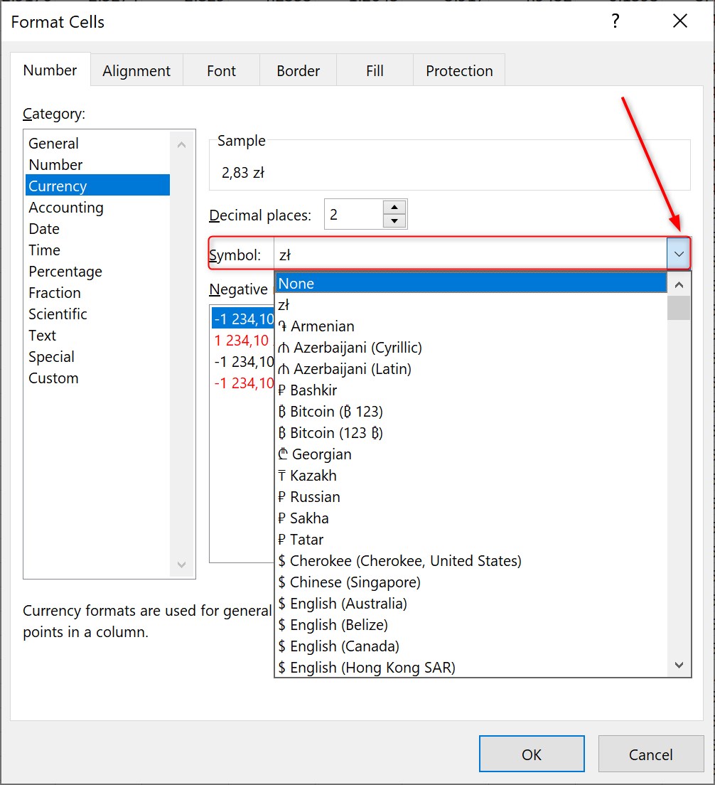
Currency and accounting format – both formats are very similar and display numerical data in monetary form. The difference is that in the case of the accounting format, we cannot choose a specific way of presenting negative numbers.
However, for both formats we can choose multiple currency symbols:
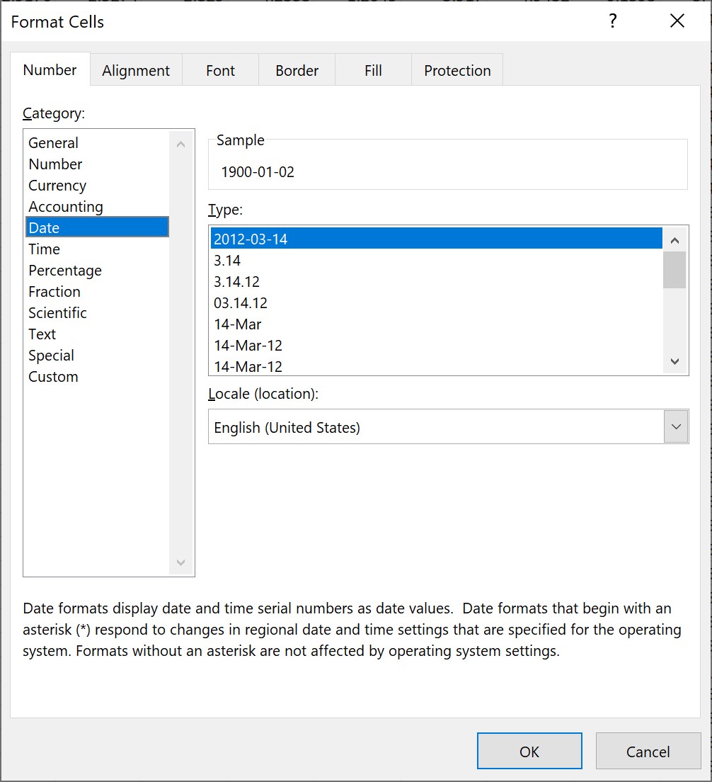
Date format – an appropriate date format can be set within this category. You can choose from various options such as long date, separating the day, month and year using a dot or dash, or changing the order of day-month-year.
Time format – a category used to define the time format. Formatting in this category is very similar to date formatting.
Percentage format – using this format causes, that data entered into the cells is converted into a percentage. After selecting this format, value entered into the cell is multiplied by 100 and the % sign is added automatically. In percentage format, you can also specify the number of decimal places:

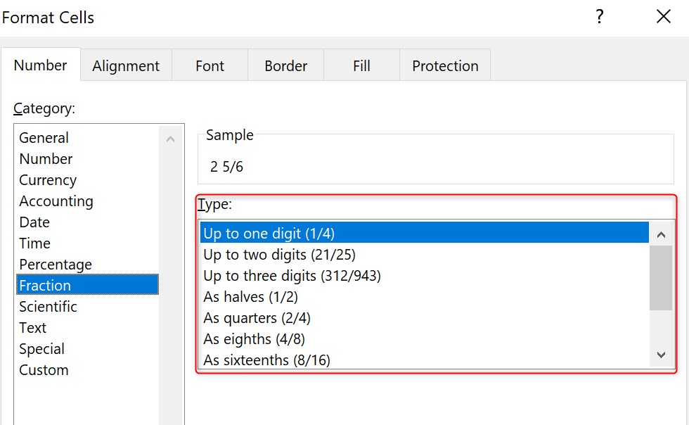
Fraction format – converts the number to a fraction with a slash “/“. There are many types of fractional form to choose from with various denominators:
Scientific format – allows you to write the entered number in exponential form and replaces the part of the number with the sign E + n, in which E multiplies the preceding number by 10 to the nth power. For example, the number 20,000 will be written as 2.00E + 04, so it means 2 * 10 to the power of 4. You can also specify the number of decimal places for this format.
Text format – this formatting causes that all data entered into a given cell will be treated as text, even if they are numbers.
Special formats – depending on the selected regional settings, allows the use of additional special formats. For USA regional settings, you will have the option of choosing such formats as Zip Code or Telephone Number.
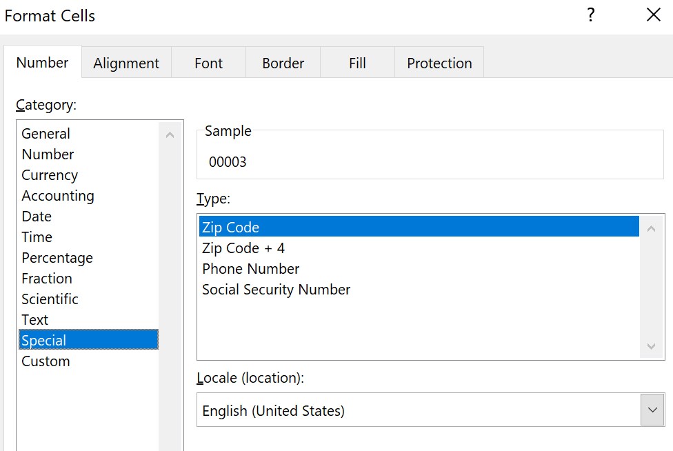
Custom formats – this is an option that allows you to create a new, custom format, in case of default available formats do not give the expected results. Custom formatting is quite complicated issue, so I am going to explain it more detail in a separate article.
You can find most commonly used data formats in the drop-down list available directly on the Home tab:
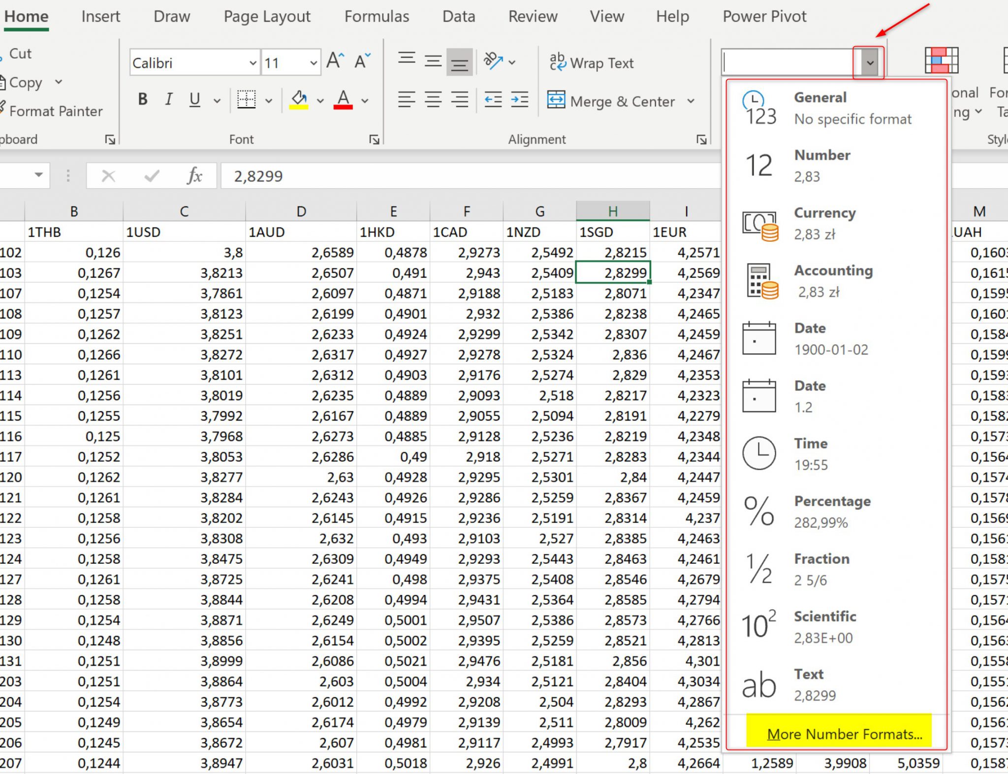
If the format you are looking for is not visible in the list, just click the More number formats command and a dialog window with detailed options for formatting data in cells will open.
Important notice:
You should remember, that changing the data format in a cell (currency, number, percentage, etc.) does not affect the actual value entered into the cell, but it only changes the way the number is presented.
Example:
All cells in row 1 contain the number 8.5, but they have different data formats set up. Cell A1 was formatted as a number, A2 as a percentage, A3 as a currency, and A4 as a fraction:

Tip:
The most popular data formats can be quickly set using keyboard shortcuts:
Ctrl + Shift + 1 – changes the format to decimal numbers;
Ctrl + Shift + 2 – sets the time format;
Ctrl + Shirt + 3 – sets the date format;
Ctrl + Shirt + 4 – defines currency formatting;
Ctrl + Shirt + 5 – modifies the format into percent.

4 thoughts on “Cells formats in Excel”