How to calculate average in Excel?

When working with numeric data, sooner or later you will need to calculate average values. In this article, I will show you basic methods of calculating average in Excel.

Command Average on the Ribbon

The first, most basic method of calculating average is Average command, which can be found on the Ribbon, under Home tab.

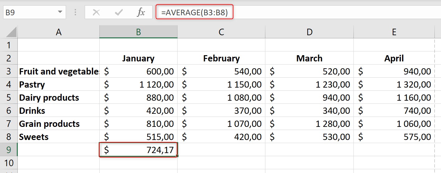
To calculate average, you need to highlight data range in a specific row or column and then click on Average button, available after clicking AutoSum. After this action, you will find new cell under highlighted column or at the right side of highlighted row with calculated average value. Additionally, you can see that AVERAGE formula has been automatically added in formula bar:

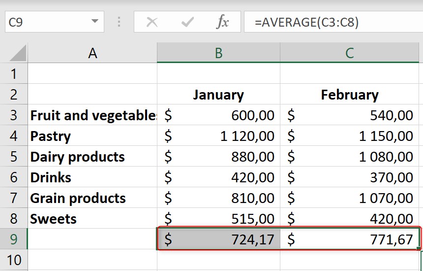
This is the easiest and fastest way, however it has some disadvantages. The main one, is the fact, that this method can be used only for data entered in one specific row or column. In case we need to calculate average value of data entered to various rows and column this way is not sufficient. You can see it on example below – after highlighting both column and using “Average” command on the ribbon, Excel calculates two separate average values for each column.

How to use AVERAGE function?

Function AVERAGE is very helpful when we need to calculate average based on data entered to more than one row and/or column.

Syntax of AVERAGE function:

=AVERAGE(Number1;Number2;…)

Number 1 – required input; this is the first number, cell or cell range for which you want to calculate average value;
Number 2;… – optional inputs; these can be additional numbers, cells or cell ranges for which you want calculate average. You can add up to 255 optional inputs.

Examples for using AVERAGE function:

=AVERAGE(B3:B8) – calculates average of values entered into cell range between B3 and B8;
=AVERAGE(C3;C5;C7) – calculates average of values entered into specific cells: C3, C5 and C7, which are highlighted in blue in this example;
=AVERAGE(B3:B8;C3:C8;D3:D8) – calculates average of values entered into three cells ranges: B3 to B8, C3 to C8 and D3 to D8. Each cell range is separated by using semicolon.

Useful Tip:
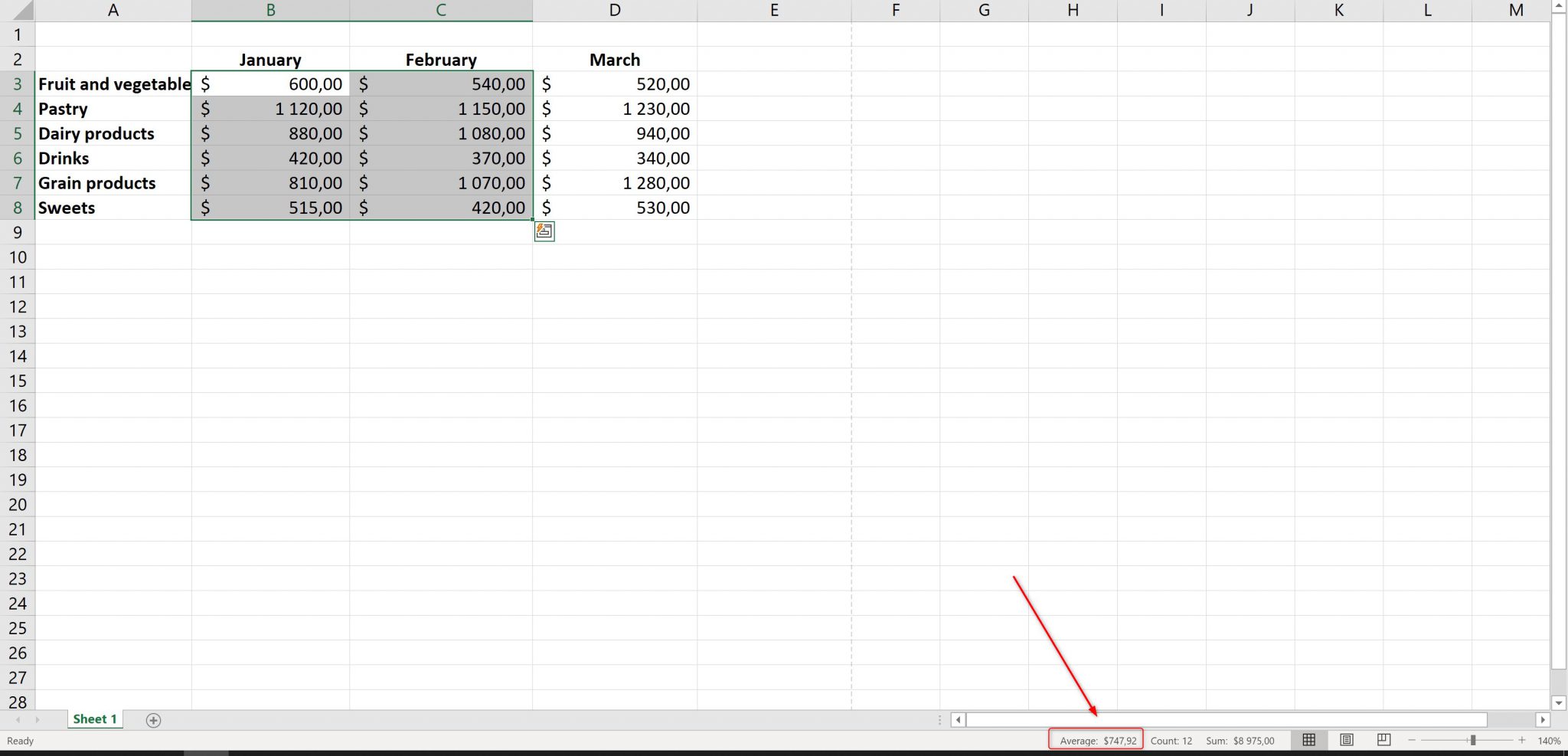
When you highlight two or more cells in Excel, some mathematic data such as sum, count and average are automatically calculated and shown on the status bar located at the bottom of spreadsheet: