Relative, absolute and mixed cell reference in Excel

Many formulas used in Excel contain references to other cells. This reference allows Excel automatically refresh formula results. To make more accurate and complex calculations you need to understand, what are cell references in Excel.

There are three types of cell references in Excel: relative, absolute and mixed.

Relative reference

Relative reference is basic and most popular cell reference type used in Excel. Example:

As you can see, cell D3 points to cells B3 and C3 – these two are relative references. If you use relative reference, address of formula will be changed when you move formula to other cell:

After dragging down formula from D3 to D8 you can notice, that in each row formula changed address: B3 and C3 has been changed to B4 and C4 in formula in row D4 etc.

Absolute reference

Absolute reference is opposite to relative one and it allows to change formula location to other cell without changing its address.

These type of reference are used when Excel spreadsheet contains some fixed values, such as interest rate or currency exchange rate. Thanks to absolute reference, Excel receives an information that it should use specific cells, regardless of where formula will be copied or entered.

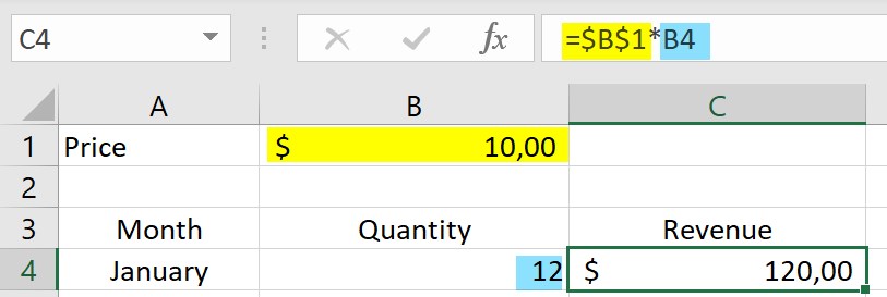
Absolute references are created by adding $ sign before column letter or row number:

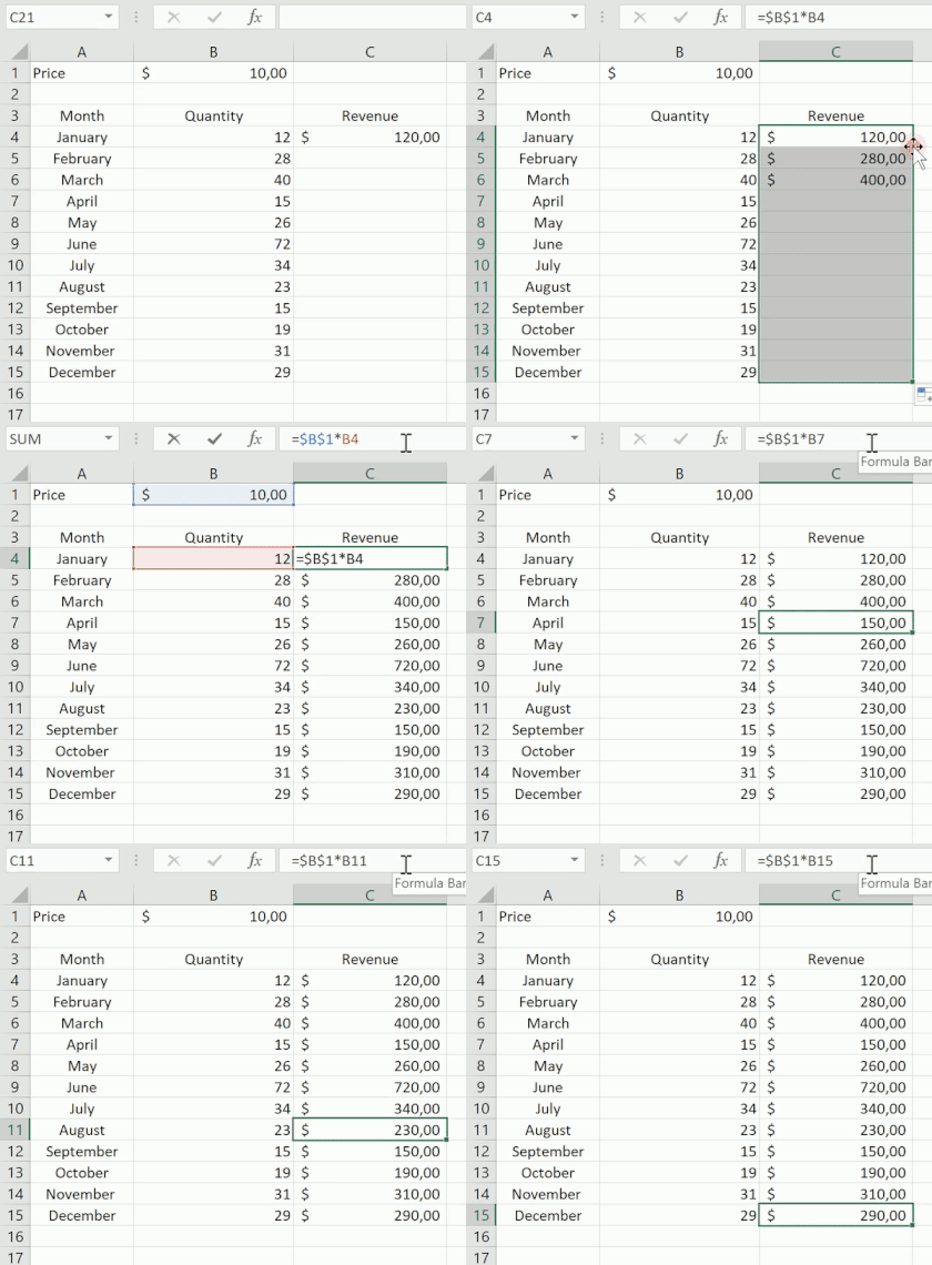
As I mentioned earlier, when we use absolute reference we can drag down or copy formulas in every place in spreadsheet without the need for manual change of formula’s elements.

Let’s see how it looks in practice. When we drag down formula from C4 to C15, it multiplies value from cell B1 by value entered into corresponding cell in column B for current row:

Mixed reference

Mixed reference consists of relative and absolute references elements and it is made by entering $ sign only before column letter or only before row number.

Examples:
$A1 – refers to column A
A$1 – refers to row 1

Mixed references are commonly used when we want to copy formulas between various rows and columns within Excel spreadsheet. Thanks to them there is no need to change manually formula’s parameters after changing its location in the spreadsheet.

Example:

We have to calculate what is the price of some products after getting 10%, 15% or 20% discount. As you can see, when we use relative reference (without $), formula moved right from D4 to F4 is not working properly:

To avoid such situation we need to use mixed reference to block column B, so address our cell as $B4:

After that change, even if we drag formula right, its first value will be always taken from cell in column B for corresponding row.

We can notice similar example while dragging down formulas. If we create mixed reference blocking only row number – D$2 – formula will calculate value entered in row 2 for current column:

Then, if we drag formula right again, we can see that it still takes the value from row 2 accordingly for columns E and F:

TIP:
You can speed up your work and use F4 key except of manual input of $ before row number/column letter.
One press of F4 – $A$1 – adds $ before column and row;
Double press F4 – A$1 – adds $ only before row number;
Triple press of F4 – $A1 – adds $ only before column letter.
When you press F4 fourth time, you will back to initial setting, so it will put $ before column and row again.