
Cleaning, editing and transforming text is very important part of work in Excel. In this article, you can find out 10 most useful and most popular text function, which will improve your work with text data in Excel.
LEFT
LEFT function in Excel returns characters from the left side of given text string based on the number of characters defined by the user.
=LEFT(text, [num_chars])
Text – text string containing character(s) to be extracted,
Num_chars – specifies, how many characters will be extracted from Text.
Example:
LEFT function used in B1 has returned 4 characters from left side of text entered in cell A1:

RIGHT
RIGHT function is very similar to LEFT, but the difference is that RIGHT function extracts characters from the right side.
=RIGHT(text, [num_chars])
Text – text string containing character(s) to be extracted,
Num_chars – specifies, how many characters will be extracted from Text.
Example:
RIGHT function used in C1 has returned 5 characters from left side of text entered in cell A1:

MID
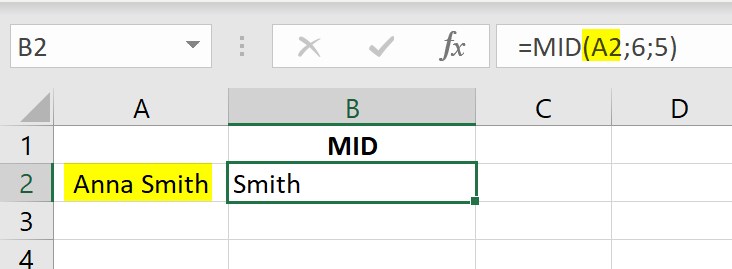
MID function returns specified number of characters from the middle of given text string, starting from the position defined by the user and based on number of characters provided by the user.
=MID(text, start_num, num_chars)
Text – text string, which includes characters to be extracted;
Start_num – defined position of first character which will be extracted from text string; for example, “3” in this argument means, that text will be extracted starting from 3rd character in given text string;
Num_chars – specifies, how many characters will be extracted starting from character defined in Start_num.
Example:
MID function in B1 has returned 5 characters starting from 6th character in text from A1:

LEN
LEN function in Excel is used to “calculate” how long is given text string. Thanks to LEN function, you can return the number of characters in a text.
=LEN(text)
Example:
LEN function calculates in B2 the length of text string in A2 – please note, that spaces are also considered as character:

SUBSTITUTE
SUBSTITUTE function in Excel is used to replace any part of the text string.
=SUBSTITUTE(text, old_text, new_text, [instance_num])
Text – argument including text or reference to a cell including text to be replaced;
Old_text – text to be replaced;
New_text – text which will be entered in place of old_text;
Instance_num – optional argument; specifies which occurrence of old_text you want to replace with new_text. If you specify instance_num, only that instance of old_text is replaced. Otherwise, every occurrence of old_text in text is changed to new_text.
Example:
Name “Anna” from text in A2 has been replaced by name “Maria”:


SEARCH
SEARCH function in Excel shows the position of first occurrence of given character(s)/text in text string, looking from left to right.
=SEARCH(find_text,within_text,start_num)
find_text – character(s) or text to be found in given text string;
within_text – this is the text you want to search and find character(s)/text defined in argument find_text;
start_num – optional argument; specifies the character number in within_text at which you want to start searching.
Example 1:
With SEARCH function, we can find out, on which position in A2 we can find letter “M”:

Example 2:
You can also find position of given word – in this example we can use SEARCH function to know, in which position in A2 we can find last name “Smith”:

TRIM
TRIM function in Excel removes all additional spaces from given text string, except for single spaces. This function is very useful, when text includes irregular spaces between words.
=TRIM(text)
Example:
In case of there is single space between words, TRIM function will not work and space will be left as it is:

However, in the situation that between name and last name there are two or more spaces, TRIM function will remove all additional spaces and leave only one:

UPPER
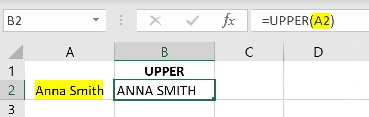
UPPER function in Excel allows to change all characters in given text to upper cases.
=UPPER(text)
LOWER
LOWER function in Excel allows to change all characters in given text to lower cases.
=LOWER(text)

CONCATENATE
CONCATENATE function in Excel is used, when two or more text strings have to be combined.
=CONCATENATE(text1;[text2];…)
Text 1, Text 2,…, – arguments of the function, they define text or data strings which should be combined. Text 1,2…, can be defined as cell references such as A2, B5 etc., but also manually entered texts.
Example:
Texts from cells A2 and B2 have been combined; additionally there is space added between these two texts:

If we don’t add a space between A2 and B2, the result will look like as below:

You can read more about combining texts in Excel here.